THERE IS A MISTAKE, PLEASE DISREGARD ANYTHING SAID HERE. I WILL FIX THIS AS SOON AS I’M DONE WITH FINALS! SORRY<3

Introduction

Last Update: 21 March 2023

This project started with an “What if” idea. The idea bein to code economic models, and inhabit them with AI agents. And see what happens 🙃!. This led me down the path, to establishing few main thing to work on. First, I need to learn how to code such model (enviroment) and allow agents to interract with it and learn to teach agents to have a meaningful interaction with the enviroment.

To kick things off, I decided to start with modeling famous in economics “Cake Eating” problem. Particularly this is a good thing to start with, because this is maybe the simpliest model in economics, but also it has a mathematical solution. This allows me to check if I’m on the right path.

Model 1. Cake eating

Into

The first “Cake Eating” model was inspired by article from QuanEcon.

The article suggests that the analytical solution for CRRA utility function is:

Where $\mathit{v}(x)$ is a lifetime be maximum lifetime utility attainable from the current time when $x$ units of cake are left. Please refer to an article for more details.

The goal of this model, is to reproduce this analytical solution purely with Reinforcement Learning techniques.

The first hurdle I ran into is that we have continous action space. As our agent can have any $x_t \in [0, c_t]$ amount of cake, where $c$ is total amount of cake at the point of time $t$ when the action is taken.

There are two ways to go around this problem:

1. First make it discrete, meaning give agents a set of choilces (which can depend on size of cake, for instance $a_t = \{ 0.1c, 0.2c, 0.5c, 0.7c \}$ where c is the size of the cake.
2. Figure out a way to implement RL learning for continous state of action.

Since about first way to solve the issue I only came up while writing this, we will proceed with second. First method also is not very reasonable, but maybe will do that in the future too.

To start things off I found this article, which creates a custom enviroment for RL model, and trains the agent similar to what I want to do in this model.

After reading the article and starting of with the 🤗 RL course, and trying to figure out waht it all means, this is what I’ve got: (Nothing Yet).

Ideas and Estimations

Before I start playing with the RL, I need to, at least estimate, what my Agent should achieve. To do so, let’s see what the agent will be doing:

Agent steps:

1. Observe action space $c_t \in (0, C_t)$, where C_t is total cake available at the moment $t$.
2. Choose action
3. Recieve reward
4. Repeat steps 1-3 until $C_t$ is small enough (it will technically never be zero)

Speaking mathematical language:

We can also say that $c_t = C_t * \alpha$, meaning that at each step Agent will eat curtain proportion of availiable cake.

This way:

If we open up the $\sum$ and see what’s happening inside, we will see:

$V(\alpha) = u(\alpha C) + u(\alpha(C - \alpha \cdot C)) + u(\alpha(C - \alpha(C - \alpha \cdot C))) + \cdot$

$V(\alpha) = u(\alpha C) + u(\alpha C - \alpha^2 C) + u(\alpha C - \alpha^2 C + \alpha^3 C) + \cdots$

Or

C - is initial amount of Cake.

Now, let’s define $u$. In the QuanEcon article they used CRRA utility function, which I will use for the purpose of this study too. Later will test other functions.

If to introduce $u(c)$ to our utility equation, we and simplify, we get: \(V(\alpha) = \frac{C^{1 - \gamma}}{1 - \gamma} \cdot \sum_{i = 1}^N \left( \sum_{j=1}^i (-1)^{j - 1} \alpha^j \right)^{1 - \gamma}\)

To make it super short, the agent needs to find such $\alpha$ to maximize $V(\alpha)$.

Before we try teach the agent to do this, let’s do some estimations:

First we need our utility function:

def utility_function(c):
    global gamma
    return c ** (1 - gamma) / (1 - gamma)

Here $c$ is chosen consumption, and y is a hyperparammeter of CRRA function.

Now let’s recreate our $V(\alpha)$:

def f(x):
    n = 1000
    sum = 0
    for i in range(1, n):
        c = 0
        for j in range(1, i):
            c += (-1) ** (j - 1) * (x ** j) * C
        sum += utility_function(c)
    return sum

Why $n=1000$, well, there are no reason to choose this exact number, obviously the larger $n$ the better, however, for larger $n$ it will take a lot more time. This function has complexity $O(n^2)$.

Now let’s find at which $x$ this function is maximized:

from scipy.optimize import minimize_scalar
C = INITIAL_CAKE

bounds = (0, 1)
res = minimize_scalar(lambda x: -f(x), bounds=bounds, method='bounded')
x_max = res.x

After some tests and waiting time, some results for $n$ (sorry for the mess, but numbers after “.” matter in this case):

At $n = 1000$ $x_{max} = 0.9822492010317977$
At $n = 2000$ $x_{max} = 0.987396714651555$
At $n = 4000$ $x_{max} = 0.9910643284534496$

The difference is quite large, so let’s try Gradient Descent and Newton Method:

def gradient_descent(f, x0, lr=0.01, eps=1e-4, max_iter=1000):
    x = x0
    for i in range(max_iter):
        grad = (f(x + eps) - f(x - eps)) / (2 * eps)
        x_new = x - lr * grad
        if abs(x_new - x) < eps:
            break
        x = x_new
    return x

x_max = gradient_descent(f, x0=0.99)
print("gradient_descent", x_max)

def newton_method(f, x0, eps=1e-4, max_iter=1000):
    x = x0
    for i in range(max_iter):
        # calculate the gradient and Hessian matrix
        grad = (f(x + eps) - f(x - eps)) / (2 * eps)
        hess = (f(x + eps) - 2 * f(x) + f(x - eps)) / (eps ** 2)
        # update x using Newton's method
        x_new = x - grad / hess
        if abs(x_new - x) < eps:
            break
        x = x_new
    return x

x_max = newton_method(f, x0=0.99)
print("newton_method", x_max)

Interestingly enough, gradient descent didn’t produce any results, but newton_methond estimated $x_{max} = 0.9822490083787816$.

This way we can estimate that our target utility for the agent is for $\gamma = 0.5$ $V_{max} = f(x_{max}) = 44251.104648398985$

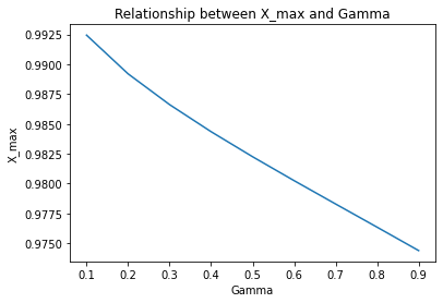
Also, with some adaptations for newton_method function, we get the following graph.

Now, that we have base line, we can start looking Agent.

Agent and RL

Model 2.

TODO

Model 3.

TODO

Model 4.

TODO

Model 5.

TODO

Model 6.

TODO

Model 7.

TODO

Model 8.

TODO